SolCalc Consulting

Bayes’ Theorem

Posted on August 3, 2017August 24, 2017 by mason.mcelroy@solcalc.com

I wanted to start off my blog with something simple to dip my feet in the water, and so I’m going to go with Bayes’ Theorem. Here it is:

$P(\theta|X) = \frac{P(X|\theta) P(\theta)}{P(X)}$

This guy is single-handedly responsible for creating an entire branch of statistics, and it so simple that its derivation is typically done in an introductory class on the topic (usually in the first couple weeks when you’re going over the basics of probability theory). It’s not until you go into more advanced classes that one realize it has a lot more to say than how big the ratio is of the cross section of circles on a Venn diagram. When I was taught Bayes’ Theorem I just thought of it as a nifty little trick for converting $P(A|B)$ statements to something that uses $P(B|A)$ . And as a student I said to myself “Cool, good enough to do my homework and pass a test I’ll never see this again.”

Fast forward 2 years later and I actually DO see it bullshit again. And surprise, it’s used for EVERYTHING. In fact, there is an entire field of mathematics dedicated to understanding its properties. It provides a new way of not just looking at statistics, or of probability, but of human knowledge! Bayes’ Theorem tells us to stop looking as our knowledge as some fixed property. The world may contain true and false statements about itself, but our knowledge about it is constantly fluctuating with new evidence, and we need to update our ideas about the world accordingly based on that evidence.

So let’s look back at the original theorem. I don’t like the way it’s usually written. Instead I’d like to make a small adjustment.

$P(\theta|X) = \frac{P(X|\theta) P(\theta)}{P(X)} = \frac{P(X|\theta) }{P(X)} P(\theta) = \text{BayesianAdjustment}(X,\theta) P(\theta)$

My little improvement on Bayes’ Theorem consists of just highlighting the little adjustment factor given by $\frac{P(X|\theta) }{P(X)}$ . I believe this little ratio hasn’t been given the right amount of credit in the current literature. If we think of $P(\theta)$ as our confidence in the belief of some statement, and $P(\theta|X)$ to be our updated level of confidence of some statement (where X is some evidence for or against that statement), then the adjustment factor should tell us exactly how much our beliefs should change.

So let’s think of $\theta$ as some statement about the world. This could be anything, like say… “Jeff Bezos is an Illuminati shill.” Now personally I don’t believe this is true, but I like to think of myself as an open minded individual so I won’t completely rule it out. I will assign the accuracy of this statement some small probability. Let’s say $P(\theta)=0.0001$ . So there is one chance in 10,000 that Jeff Bezos is definitely an Illuminati shill.

So how can you tell if someone is actually working for the Illuminati? Well, every once in a while they’ll throw out a hand signal (sort of like a low key gang sign). See exhibit A:

Capture

So one day Jeff Bezos is giving a keynote address and he decides to sit down. Lo and behold the camera gives him a quick glance and this creep is throwing out this ungodly hand sign, signaling his complicity in a hostile world-takeover by our Satanic overlords. Or he could’ve just randomly rested his hands there for no particular reason (like I said, I’m open minded). Let’s assign a value to these two possible explanations….

Let’s call the act of giving the hand signal our evidence $X$ . Then in general the probability of Bezos giving out the hand signal if he is an Illuminati member is $P(X|\theta)=1.0$ , and the probability of him putting his hands there (for no particular reason) is $P(X) = 0.2$ . Looking at these numbers by themselves the evidence seems pretty damning, but we still haven’t considered our prior assumptions about Jeff Bezos. Initially we pegged his odds of being a devil-worshipper at 1 in 10,000. Let’s plug all these into Bayes’ Theorem and see what should be our updated confidence in Jeff Bezos’ Illuminati complicitness should be, given this new piece of evidence…

$P(\theta|X) = \frac{P(X|\theta)}{P(X)} P(\theta)= \frac{1.0}{0.2} \times 0.0001= 0.0005$

Well, I definitely think he’s more likely to bring about the New World Order than I did before, but not by a significant enough margin to spout apocalyptic nonsense via HAM radio…

I could go on and on about this wonderful little equation. I can talk endlessly about how it is the most powerful epistemological statement in modern philosophy. But the fact is: you already use it in your every day life. Perhaps not as precisely as you should, but you are using it loosely every time your beliefs change. Every time you are presented some piece of evidence about the world and what is happening with it. Every time you’re not sure if Bitcoin is a good value after the last dip, or when you’re absolutely confident that all pickles taste like ass after your hundredth try. Next time you’re reading a news article think about how your beliefs are being updated, and to what degree and why.

Now I’d like to ask the reader: When was the last time you changed your mind about something? Can you assign numbers to your beliefs? If you would like to go beyond what I discussed, try asking yourself how robust your inferences are. How much do your posterior beliefs change based on your prior assumptions? Change up your values and come up with a basic “sensitivity” analysis.

Let me see what you come up with!

-Mason

Introduction to Mathematical Interpretations

Posted on August 1, 2017 by mason.mcelroy@solcalc.com

Allow me to wax poetic for a little bit. Mathematics is like poetry: it is the art of conveying an idea in as efficient and concise a manner as possible. A beautiful equation can convey mountains of ideas in a single line, and to read and understand all of those ideas can take a few seconds or it can take a lifetime.

The purpose of this blog will be to unravel some of the mathematical statements I have come across, and interpret them in a way that I hope will be enlightening and enjoyable to others. The math I tend to enjoy generally comes from the fields of analysis, statistics and applied mathematics (some ideas I have for initial equations I would like to dive into include Bayes’ Theorem, Fisher Information, and the Kelly Criterion).

One final note: Unlike a poem we don’t think of mathematics as aesthetically pleasing. I hope that by writing my ideas behind equations I can demonstrate, just like with a haiku, how beautiful a small little statement can be.

-Mason McElroy

Evaluating Player and Team Offense

Posted on September 21, 2016August 23, 2017 by mason.mcelroy@solcalc.com

What I propose is a first attempt at developing a mathematical model for evaluating a team of five players. There are assumptions within this model that are unrealistic, but I believe that progress can be made towards tackling these assumptions in the future.

The idea is directly inspired by the player shot charts which were popularized by Kirk Goldsberry during his time at Grantland.

What if we could summarize this data into a single number? We would lose a lot of the spatial details of where certain players and teams are most effective, but in turn we could have a new metric to compare (and hopefully predict) player and team offenses.

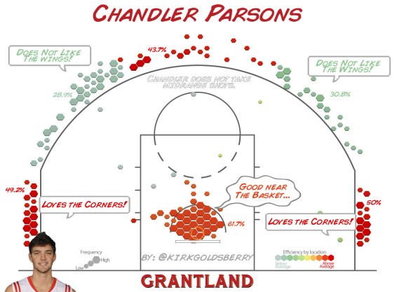
Let $n$ represent the number of players in the league, and let each player in the league be indexed by $i$ , where $1\leq i\leq n$ . Furthermore, let the expected point value of player $i$ at position $(x,y)$ on the court be represented by $EV_i(x,y)$ . Then we’ll define the player’s total offensive value as

$TO(i) = \int_\mathbb{C} EV_i(x,y)\times p_i(x,y) d(x,y)$

Where $mathbb{C}$ represents the two dimensional court space, and $p(x,y)$ represents the probability at which player can get to position $(x,y)$ . So $TO(i)$ represents the value of player $i$ on the entire court.

We can use this metric to define the best offensive player in the league. i.e. The best offensive player is defined by the index $i$ that maximizes $TO(i)$ .

Defining the value of a player on offense is interesting by itself, but limiting. We can extend this model to look at the best 5-player offence. Let $I\subset {1,...,n}$ be a 5-tuple, where each element is different. This will represent 5 different players in the league. Then the value any 5-team offense at any position on the court can be represented by $\max_{i\in I} EV_i(x,y)\times p_i(x,y)$ . That is, the value of the team at position $(x,y)$ is the value whichever player has the best expected value at position $(x,y)$ . Similarly, the total team offense can be represented as

$TTO(I) = \int_\mathbb{C} \max_{i\in I} EV_i(x,y)\times p_i(x,y) d(x,y)$

With this formula we have a foundation to evaluate arbitrary team offenses. However there is still the decision on how to represent $EV_i$ in a manner that is both calculable and useful.

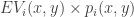
For now let us represent $EV_i$ as the expected number of points a player will score. This can be easily estimated based on a player’s sample performance at various points along the court. However, this doesn’t give us a complete picture of a player’s value on offense. Things get messy when we want to integrate something as simple as an assist, since it is also dependent on the other five players on the court. Then there are roles that a player performs that are even more difficult to assign value for, such as setting a screen or spreading the defense. For now we’ll have to settle for a more simplistic approach and hopefully tackle these other issues in the future. With this assumption we can estimate $EV_i(x,y)\times p_i(x,y)$ using standard kernel density estimation techniques.

A programmatic implementation will come soon.

Home Court Advantage in the NBA

Posted on September 18, 2016 by mason.mcelroy@solcalc.com

We’ll start this blog with a basic overview of home-court advantage (HCA). It is commonly accepted that the home team will have an advantage over the visitors in any sport, and basketball is no exception. There are several possible reasons why HCA may manifest itself: Officiating bias, crowd support, travel… Whatever it may be, the cause shouldn’t stop us from analyzing the effect. We wish to explore what the value of playing at home is, as well as look at possible trends in playing at home.

If we were to count the +/- point differential for home teams over the last decade it would look like this: differentialhisto

This histogram holds some interesting information. For example, it’s worth noting that it’s more likely to win or lose a game by 10 points than by 1 point. But that is an anlalysis for another time. What we’re interested in is the blue line.

The blue line represents the average HCA. The data may look noisy around the mean, but thankfully we have enough data to conclude that we can’t attribute this 2.93 point advantage to simple random variation:

The conclusion we can come to is that the home team has an advantage that can be compared to roughly one extra made 3-pointer every game. Though it may not manifest itself in a way that’s as exciting as a clutch game winner, it is still a very real phenomenon.

With this knowledge we may also wish to know more about HCA. Specifically, we can look at whether not it benefits specific teams more than others. Consider the data from the 2015-2016 season.

Interestingly enough, the Minnesota Timberwolves had a better scoring differential on the road than they did at home last year. Furthermore, based on this data, one may conclude that Detroit and Portland have the best HCA in the league. However, this isn’t enough to suggest a real advantage for specific teams. What if Portland’s #1 ranked scoring differential can be explained by random variation? After all, someone has to be first.

Consider the data from the previous season.

The biggest change in HCA would belong to the Orlando Magic, going from lowest to 3rd highest in one season. Exploring the data even further back, it is difficult to find any trend in HCA by team. I am personally skeptical that a measurable advantage exists.

The final item I’ll look at is HCA over the years.

There doesn’t appear to have been any discernible change in HCA over the last decade. If one were to believe that officiating has improved over the years, then we can remove officiating bias from our assumption that it benefits the home team. Instead, it may be something more abstract. The energy and support of a home-crowd may have a powerful effect on both teams, whether psychological or physiological. Whatever may be the cause, it looks like it’s here to stay.

Note: R code can be found here.

Pokemon Go Fading?

Posted on August 26, 2016 by mason.mcelroy@solcalc.com

http://fivethirtyeight.com/features/our-national-love-affair-with-pokemon-go-might-be-short-lived/

While the drop off is interesting by itself, I think you lose part of the story by not comparing the active users over time with other popular F2P games. What I want to know is, is a 30% drop-off within the first month of release unusual? Is that small or large in context? I have no idea.

The only problem with investigating this question is that there’s really no other game like Pokemon Go to compare it to. The closest I’m aware of is Ingress, but that doesn’t have nearly the same historic brand-loyalty associated with it. I still think it would be a useful comparison, though.