mason.mcelroy@solcalc.com

Book Recommendation: Addiction By Design

Posted on May 29, 2025 by mason.mcelroy@solcalc.com

An early mentor recommended this book to me as a budding young slot designer and ever since it’s informed how I think about game design. It’s written as a critique of the casino game industry and an exposé of their left-hand tactics. I use it as a how-to guide.

My favorite takeaway is the idea of what I call a flow state (the book calls it the Machine Zone). My design philosophy emphasizes removing confusion, awkward pauses, information overload, decision making, and anything that could distract or disrupt the flow state.

Even if you’re not interested in the design aspect of casino games, it’s the best overview of the industry that I’m aware of. Would highly recommend it to anyone wishing to learn more about what we do, and how it all works.

Choosing a Game Theme

Posted on February 11, 2022June 17, 2025 by mason.mcelroy@solcalc.com

Scott Adams, the creator of the Dilbert comic strip, explained why animated adaptation of his comic failed. Fans of the comic didn’t watch the cartoon because they disliked Dilbert’s voice—a small detail that alienated them.

Comics like Dilbert thrive because they don’t tell the reader much. We don’t know Dilbert’s last name, address, job title, or what his company does. His boss is simply “The Boss.” This vagueness lets readers project their own experiences onto the characters.

Similarly, the most successful casino games rely on broad, simple themes:

Generic Chinese theme
Generic Egyptian theme
Generic Greek theme
Jewels
Strong animals
Sexy characters

These themes are deliberately sparse, offering just enough context to engage without overwhelming players. Too many details risk alienating the audience.

Take the game Crash as an example. A rocket and a number rise, and you cash out before it crashes. That’s it. Would it be as popular if we knew who was in the rocket, where it’s going, or why? Probably not. Simplicity keeps players hooked.

Less detail often means more connection. Whether in comics or games, leaving room for imagination drives engagement.

Measuring Casino Game Volatility

Posted on February 19, 2021May 12, 2021 by mason.mcelroy@solcalc.com

Standard Deviation

When we think about the volatility of data, the first concept that comes to mind is the almighty standard deviation metric. This is a good metric for 99% of casino games on the market, but over the last 5 years or so we’ve started to see a new class of game emerge: persistent state games (think games like Scarab or Ocean Magic). What happens in these games is bets are not independent. Instead some characteristic of the game carries over from one bet to the next, usually resulting in large wins at somewhat regular intervals.

The violation of bet independence makes standard deviation a lackluster metric for assessing the volatility of these kinds of games. The regularity of these large wins results in a deceptively large impression of the game’s volatility. Can you say a game is volatile if your typical player gets a lot of time on device?

A Better Metric

I propose a much more effective metric for volatility that works for this emerging class of games, as well as more traditional casino games: Median Spins (or Median Bets). The idea is to capture how long it takes the typical player to exhaust their bankroll. The more bets a typical player is able to make on a game, the less volatile it is. You can visualize how volatility affects median spins by comparing the histograms below.

**Left**: Less volatile. **Right**: More volatile.

How to calculate median spins

Unfortunately for most games there’s no simple formula for determining median spins, but it’s easy enough to determine it via simulation.

Start by running a full game simulation where a player starts with a bankroll of 50 times the cost to cover (for a 40 cent game this would be $20).
Determine how many bets it takes for the players to exhaust their bankroll. For calculating median spins you can usually cap this metric at 1000 spins to save simulation time.
Repeat this process X times, keeping a log of how many spins it took each player to exhaust their bankroll.
Finally, calculate the median value from the data to determine median spins.

In my experience, if we start with a bankroll of 50 times the cost to cover, median spins of less than 100 could be considered a high volatility game, and median spins higher than 150 would be considered low volatility.

Average Spins?

In case you’re curious, average spins is an absolutely useless metric for measuring anything, except for maybe reverse engineering the RTP of a game. This is because the average number of spins is completely determined by the RTP of a game. Imagine the player has enough to cover a single bet on a game. On average how many spins will this single bet give you?

This is a geometric series with a known solution. From here we can just plug all the known values into the following formula.

If a player starts with a bankroll 50 times the cost to cover, and the game has a 90% payback, then on average they’ll get 500 spins out of the game regardless of the game’s volatility.

Assessing Fake News: An Information Theoretic Approach

Posted on October 16, 2020May 9, 2025 by mason.mcelroy@solcalc.com

In 1948 Claude Shannon published a landmark paper that gave rise to a new field of science: Information theory. A few years ago I also published my not-so groundbreaking post on how we can make inferences from biased sources of information. I’m going to follow up that post by assessing the quality of a news source by using one of the key insights of Shannon’s research.

Let’s say you have a random source of information. The probability that it outputs a given message $x$ is given by $p(x)$ . Furthermore, let’s say we wish to construction a function, $s(x)$ , that indicates how surprising a given message is. How might you want to construct such a function? An intuitive approach might be to give a few constraints on things we want from $s(x)$ .

$s(x)$ decreases as $p(x)$ increases. The more likely an event, the less surprsing it is.
If $p(x)=1$ , then $s(x)=0$ . A event that is certain should yield no surprise.
As $p(x)\rightarrow0$ , then $s(x)\rightarrow\infty$ . The surprise of an message knows no bounds.

One such function that satisfies these conditions is

$s(x) = \log \frac{1}{p(x)}$ .

From here we can go a step further and measure the average surprise of a source (aka the Shannon Entropy) given by

$H(X) = E[s(X)] = \sum p(x) \log \frac{1}{p(x)}$

If we take this formula in its most literal sense it seems to reinforce our own intuitions about the quality of a news source. If a news source is always pro or anti one side or the other then it’s Shannon entropy is 0. i.e. There is no information to be gleaned from the signal. But if it occasionally surprises us then $H(X)>0$ . In fact, $H(X)$ reach its maximum when all messages are equally likely.

Do you buy this literal interpretation of Shannon’s equations? If not, do you think it can be adjusted somehow?

Investigating the Pareto Distribution

Posted on October 4, 2020October 9, 2020 by mason.mcelroy@solcalc.com

During my graduate degree program in Statistics I needed to know the ins and outs of many different probability distributions. This includes the normal, binomial, beta, gamma, exponential, and Poisson. Surprisingly I never ran into one of the most popular distributions in popular culture: the Pareto distribution.

You may have heard of the 80/20 rule? Most commonly you hear about 80% of the wealth is controlled by 20% of people. Maybe 99% of book sales are generated by 1% of authors? These numbers don’t need to add up to 100%. We could just as easily say 70% of productivity comes from 10% of workers, or 90% of your musical abilities is generated from 30% of your practice. But no matter how you slice it there’s a sense of skewness of how some percentage of input generates a disproportionate amount of output. My goal in this post is to mathematically describe how the Pareto distribution arises from simple assumptions, and how it captures this skewness phenomenon.

Let’s describe a real life property, such as a random individual’s age, via a random variable $X$ . Assume $X\sim Exponential(1)$ . That is $X$ follows an exponential distribution with PDF and CDF

$f_X(x) = e^{-x}$ and $F_X(x) = 1-e^{-x}$ for $x\geq 0$ .

From here let’s assume that everyone’s income grows over time at a constant rate of return. Ignore units and just assume everyone starts life on equal footing with a net worth of 1. Then we’ll use $Y=e^{\alpha x}$ to describe a random individual’s net worth, where $\alpha$ is the rate of return. The CDF of Y is derived like so…

$\begin{aligned} F_Y(y) &= P(Y<y) \\ &= P(e^{\alpha X} < y) \\ &= P(X < \frac{1}{\alpha} \ln y) \\ &= F_X\left(\frac{1}{\alpha} \ln y\right) \\ &= 1-\left(\frac{1}{y}\right)^{\frac{1}{\alpha}} \text{ for } y\geq 1. \end{aligned}$

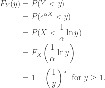
The PDF comes from taking the derivative of the CDF. We have…

$f_X(x) = \frac{1}{\alpha} y^{-(1-\frac{1}{\alpha})} \text{ for } y\geq 1$ .

This is the Pareto distribution (typically parameterized to remove the reciprocal of $\alpha$ ).

Consider $p=1-F_Y(y_0)$ . This value tells us the proportion of the population that makes an income above $y_0$ . A natural question to ask is how much wealth does this portion of the population control? To answer this question first let’s calculate the following quantities.

$\begin{aligned} \text{Total Wealth} &= \int_1^\infty y f_Y(y) dy = \frac{1}{1-\alpha } \\ \text{Total Wealth Above } y_0 &= \int_{y_0}^\infty y f_Y(y) dy = \frac{y_0^{1-\frac{1}{\alpha }}}{1-\alpha }\end{aligned}$

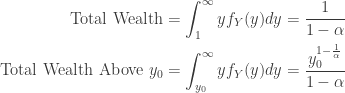
Taking the ratio of the above terms we can define a new function, $W(p)$ , to get the proportion of wealth owned by the top p percentile of the population.

$W(p) =y_0^{\frac{\alpha -1}{\alpha }} = p ^{1-\alpha}$

where the following substitution is applied

$y_0 = F_Y^{-1}(1-p) = p^{-\alpha}$ .

Now let’s consider finding a value $\alpha$ that expresses the most popular form of the Pareto Principle, i.e. the 80/20 rule. Simply setting $W(p) = \frac{4}{5}$ and $p = \frac{1}{5}$ we solve and get $\alpha =\log_5(4) \approx 0.8616$ .

In our every day world 86% may seem like an unrealistic rate of return, but keep in mind that we never gave units for our underlying distribution of age. If the units $X$ are in decades and you assume a person lives only 10 years on average, then you achieve this same level of inequality with just a 9% annualized rate of return. Of course this model is highly simplified since human lifespans don’t follow an exponential distribution with a 10 year mean. Still, it speaks volumes to how inequality can arise from something as innocuous as age and a modest return on investment.

Oddly enough there’s nothing special about the Pareto distribution that is unique in capturing this sense of inequality. We could have used this same methodology for many distributions. A natural question then becomes how $\alpha$ must change to capture the 80/20 rule when you assume a different underlying distribution for age besides the Exponential distribution.