Standard deviation is the most commonly used metric for measuring the volatility, or spread, of data. Besides mean average, it is the most commonly used metric in data science to the point where we never stop to think about why it’s used.
The formula for standard deviation is given by:

Not the simplest formula, but it does its job in capturing how data deviates from its mean. Except there is a simpler, more intuitive formula available to us. This metric is called Mean Absolute Deviation (or MAD for short). The formula looks like this:
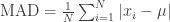
If you want to know how spread out your data is, doesn’t it make more sense to find the mean, then take the average distance of all the data from that mean? I see no reason why not.
So why is standard deviation the industry standard for measuring spread? I think it’s partly an accident of history, and partly due to the fact that square functions are easier to work with in mathematics (and lead to nicer advanced results).
Compare the square function to the absolute value function below.


Calculus has no way of dealing with that sharp corner on the right.
Okay, so we can see that there are alternatives to standard deviation. What difference does it make when analyzing data?
The consequences of using a 2nd order (or higher) polynomial when measuring spread is that data points further from the mean are weighted higher. Consider the comparison of the two data sets below:

MAD is constant between the two, but standard deviation INCREASES if we included data points that are further out.
Is this good or bad? It just depends on what you’re looking for. Are you more interested in detecting possible outliers between two data sets? Use standard deviation. More interested in how the data deviates from the mean? Give MAD a try.


 to be the event that a red ball is picked from the urn on the
  draw. So
  would be interpreted as the probability of picking a red ball on the first draw.
 and
and  . For the second probability, we consider the case where the red ball is picked on the 2nd or 3rd draw (possibly both). Which probability do you suppose is greater? Think about this question for a second before continuing reading.
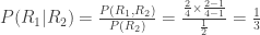

 . This result clashes with my own intuition. I would expect that knowledge of a red ball picked on the 2nd or 3rd draw would reduce my chances of having picked a red ball on the 1st draw, especially since
  includes the possibility of both red balls being selected on the 2nd and 3rd draws. How is it that the knowledge of a red ball possibly being drawn in an additional spot actually increases our odds of selecting it on the first draw?
 reduces the number of red balls available for the first draw by one, and it reduces the number of balls in the urn available for the first draw by one, giving
  . The information [
  , we should think of
  , where
  is the expected number of red balls removed when we know that the 2nd, 3rd, or both picks possibly withdrew a red ball. Let’s do that:

 . This is simply the set of all the states the player can be in.
 . i.e. What is the initial probability of being in each state?
  row vector.
 . Each element of
  to state
  would be given by the
  column of
  at each step in the process:
 step of the process.
![X_0 = \left[\frac{1}{3} \ \frac{1}{3} \ \frac{1}{3} \ 0 \right]](https://s0.wp.com/latex.php?latex=X_0+%3D+%5Cleft%5B%5Cfrac%7B1%7D%7B3%7D+%5C%C2%A0+%5Cfrac%7B1%7D%7B3%7D+%5C+%5Cfrac%7B1%7D%7B3%7D+%5C+0+%5Cright%5D&bg=ffffff&fg=333333&s=0&c=20201002)
![T = \left[\begin{array}{cccc}\frac{1}{8} & \frac{3}{8} & \frac{3}{8} & \frac{1}{8} \\ 0 & \frac{1}{4} & \frac{1}{2} & \frac{1}{4} \\0 & 0 & \frac{1}{2} & \frac{1}{2} \\0 & 0 & 0 & 1 \\ \end{array} \right]](https://s0.wp.com/latex.php?latex=T+%3D+%5Cleft%5B%5Cbegin%7Barray%7D%7Bcccc%7D%5Cfrac%7B1%7D%7B8%7D+%26+%5Cfrac%7B3%7D%7B8%7D+%26+%5Cfrac%7B3%7D%7B8%7D+%26+%5Cfrac%7B1%7D%7B8%7D+%5C%5C+0+%26+%5Cfrac%7B1%7D%7B4%7D+%26+%5Cfrac%7B1%7D%7B2%7D+%26+%5Cfrac%7B1%7D%7B4%7D+%5C%5C0+%26+0+%26+%5Cfrac%7B1%7D%7B2%7D+%26+%5Cfrac%7B1%7D%7B2%7D+%5C%5C0+%26+0+%26+0+%26+1+%5C%5C+%5Cend%7Barray%7D+%5Cright%5D&bg=ffffff&fg=333333&s=0&c=20201002)
![X_n = X_0 T^n = \left[\frac{1}{3} \ \frac{1}{3} \ \frac{1}{3} \ 0 \right] \left[\begin{array}{cccc}\frac{1}{8} & \frac{3}{8} & \frac{3}{8} & \frac{1}{8} \\ 0 & \frac{1}{4} & \frac{1}{2} & \frac{1}{4} \\0 & 0 & \frac{1}{2} & \frac{1}{2} \\0 & 0 & 0 & 1 \\ \end{array} \right]^n = \left[ p_{1,n} \ p_{2,n} \ p_{3,n} \ p_{4,n} \right]](https://s0.wp.com/latex.php?latex=X_n+%3D+X_0+T%5En+%3D+%5Cleft%5B%5Cfrac%7B1%7D%7B3%7D+%5C%C2%A0+%5Cfrac%7B1%7D%7B3%7D+%5C+%5Cfrac%7B1%7D%7B3%7D+%5C+0+%5Cright%5D%C2%A0+%5Cleft%5B%5Cbegin%7Barray%7D%7Bcccc%7D%5Cfrac%7B1%7D%7B8%7D+%26+%5Cfrac%7B3%7D%7B8%7D+%26+%5Cfrac%7B3%7D%7B8%7D+%26+%5Cfrac%7B1%7D%7B8%7D+%5C%5C+0+%26+%5Cfrac%7B1%7D%7B4%7D+%26+%5Cfrac%7B1%7D%7B2%7D+%26+%5Cfrac%7B1%7D%7B4%7D+%5C%5C0+%26+0+%26+%5Cfrac%7B1%7D%7B2%7D+%26+%5Cfrac%7B1%7D%7B2%7D+%5C%5C0+%26+0+%26+0+%26+1+%5C%5C+%5Cend%7Barray%7D+%5Cright%5D%5En+%3D+%5Cleft%5B+p_%7B1%2Cn%7D+%5C+p_%7B2%2Cn%7D+%5C+p_%7B3%2Cn%7D+%5C+p_%7B4%2Cn%7D+%5Cright%5D+&bg=ffffff&fg=333333&s=0&c=20201002)
 , you can take a look at
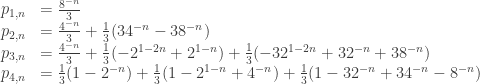
  represents the probability of being in state
  . Note that based on the above equations it is clear that
  , implying that the game is guaranteed to end given enough time. A few more interesting properties of this game can be uncovered by analyzing these equations. For example, on average, how many rounds of this game can the player be expected to play?

 be a convex function and
  be an arbitrary random variable. Then
![f(\mathbb{E}[X]) \leq \mathbb{E}[f(X)]](https://s0.wp.com/latex.php?latex=f%28%5Cmathbb%7BE%7D%5BX%5D%29+%5Cleq+%5Cmathbb%7BE%7D%5Bf%28X%29%5D&bg=ffffff&fg=333333&s=0&c=20201002)
